
Introduction
ORCHIDEE is the land surface model of the IPSL (Institut Pierre Simon Laplace) Earth System Model. Hence, by conception, the ORCHIDEE model can be run coupled to a global circulation model (Fig 1a). In a coupled set-up, the atmospheric conditions affect the land surface and the land surface, in turn, affects the atmospheric conditions. Coupled land-atmosphere models thus offer the possibility to quantify both the climate effects of changes in the land surface and the effects of climate change on the land surface. However, when a study focuses on changes in the land surface rather than on the interaction with climate, ORCHIDEE can be run off line as a stand-alone land surface model (Fig 1b). The stand-alone configuration receives the atmospheric conditions such as temperature, humidity and wind, to mention a few, from the so-called ‘forcing files’. Unlike the coupled set-up, which needs to run at the global scale (but with the possibility of a regional zoom), the stand alone configuration can cover any area ranging from the global domain to a single grid point.
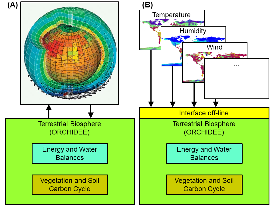
Figure 1 Conceptual differences between (A) a coupled simulation and (B) an off-line simulation. Note the same model is used and the difference is in the interface and the source of the forcing data. In the coupled set-up the interface supports a two-way interaction and the climate conditions are calculated by a global circulation model. In the off-line set-up a one-way interface is used and the climate conditions are read from forcing files.
Modelled processes
The processes included in the early versions of ORCHIDEE were aimed at quantifying the terrestrial water (Fig. 2a) and the energy balance (Fig. 2b). Later versions of the model were extended with biogeochemical processes (Fig 2c), and the current version simulates the interference of anthropogenic activities with natural biogeochemical processes (Fig 2d). The biophysical process include latent (denoted ‘evaporation and transpiration’ in Fig 2a or LE in Fig 2b), sensible (denoted H in Fig 2b), and kinetic energy exchanges at the surface of soils (G in Fig 2b). Heat dissipation and water fluxes are vertically distributed in the soil (‘drainage’ in Fig. 2a and G in 2b) and the runoff (Fig 2a) is collected in rivers and lakes. The simulated processes that affect the global carbon cycle (Fig 2c) include photosynthesis, carbon allocation, litter decomposition, soil carbon decomposition, maintenance and growth respiration and vegetation dynamics. The anthropogenic interference (Fig 2d) includes land cover changes, fire, crop irrigation, and forest and grassland management.
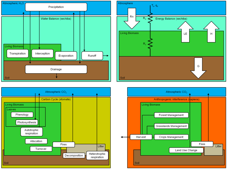
Figure 2 The main processes simulated in ORCHIDEE. The processes are grouped in terms of the water balance (a), the energy balance (b), the biogeochemical processes (c) and anthropogenic processes (d). Although the water and energy budget were separated in this presentation, both need to be run at the same time. These processes are coded in a group of modules called ‘Sechiba’ and are the backbone of ORCHIDEE. In addition to Sechiba, the biogeochemical code and the anthropogenic code, grouped in modules called ‘Stomate’, can be activated. Several individual processes can be switched on or off, so supporting a wide range of model set-ups. Nevertheless, the model can be run without activating Stomate.
Input data
ORCHIDEE calculates its prognostic variables (i.e. a multitude of C, H2O and energy fluxes) from the following environmental drivers: air temperature, wind speed, solar radiation, air humidity, precipitation and atmospheric CO2 concentration. In off-line mode, the user should provide these drivers, and ORCHIDEE simulates their impact on ecosystem production, ecosystem respiration, the energy budget of ecosystems, the soil water budget and the surface run–off at a wide range of temporal and spatial scales (Fig. 3). When coupled to an atmospheric model, ORCHIDEE follows an implicit approach. The prognostic variables of ORCHIDEE at each timestep are therefore simultaneously calculated with the atmospheric drivers in the planetary boundary layer (Fig. 1a). For both setups, the user needs to provide files describing the boundary conditions, namely the (initial) vegetation distribution (that may change with time if the dynamic vegetation module is activated) and a soil map. When the biogeochemical processes are not activated, the leaf area index (LAI) of the vegetation is read from a map, which needs to be provided by the user. When the runoff is routed through rivers and lakes, a basin and a floodplain map are required. Finally when irrigation is applied, it needs to be prescribed by an irrigation map.
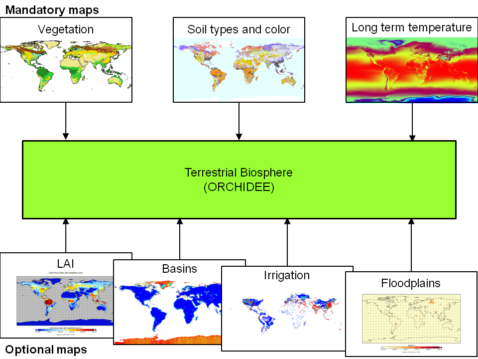
Figure 3 Mandatory (top row) and optional (bottom row) boundary conditions that need to be provided for ORCHIDEE simulations. The vegetation map specifies the location and share of the different meta-classes (13 in total), the soil types and colour map is required for soil water and energy computations as well as the calculation of the bare soil albedo. The long term temperature is required for phenological initializations. The optional maps are needed only when specific modules are to be used.
Spatial conceptualization
Although ORCHIDEE does not enforce a spatial or temporal resolution, the model does use a spatial grid and equidistant time steps. The spatial resolution is an implicit user setting that is determined by the coarsest resolution of the forcing data (Fig. 1b) and the boundary conditions (Fig 3): the vegetation distribution (default 5kmx5km), climatological forcing data (default 1°x1°) and the soil map (default 0.5°x0.5°). If higher resolution drivers are available the model can then be run at that scale. If site-level drivers are available then simulations at the site scale are feasible. When ORCHIDEE is used in a coupled set-up the grid applied by the atmospheric model determines the spatial resolution of the surface layer model (Fig 1a). For global simulations a typical grid is 2.5° latitude by 3.0° longitude.
The standard version of ORCHIDEE builds on the concept of meta-classes to describe vegetation distribution. By default it distinguishes 13 such meta-classes (one for bare soil, eight for forests, two for grasslands and two for croplands). Each meta-class can be subdivided in an unlimited number of Plant functional types (PFTs). By default, each meta-class has a single PFT. Biogeochemical and biophysical variables are calculated for each PFT (Fig 4a), where most of the biogeochemical variables are reported at the PFT level, the biophysical variables are aggregated at the pixel level because the atmospheric model does not distinguish PFTs and hence its spatial resolution is limited to the pixel scale.
For the water and heat balance of the soil, three soil columns are distinguished: one containing each meta-class that includes forest, one for every meta-class with grass and crops and, finally, one for bare soils. Water and heat related soil variables are calculated separately for each column.
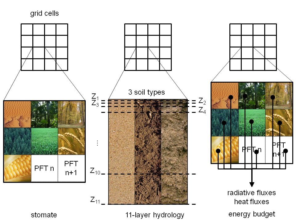
Figure 4 Spatial conceptualization of ORCHIDEE. ORCHIDEE is run at a regular grid, hence, its basic spatial unit is a grid cell, a grid cell having a known longitude and latitude. (a) The vegetation within a grid cell can be composed of 13 different meta-classes and an unlimited number of PFTs (Plant Functional Types) within each meta-class. Meta-class and PFT have no known location within a grid cell – they simply take up a share of the grid cell. The biogeochemical soil processes such as litter decomposition follow the meta-class based subdivision. (b) A similar concept is used to model the biophysical soil processes such as soil water and heat storage, however, three columns cutting across several meta-class are now used. One column is saved for the soil under tall vegetation (i.e. all meta-classes containing forest), one for short vegetation (i.e. meta-classes that contain grass and crops) and one for soil without vegetation. The three different soil columns do not have a known location within the grid cell.
Temporal conceptualization
ORCHIDEE can run on any temporal resolution, however, this apparent flexibility is rather restricted as the processes are formalized at given time steps: half-hourly (i.e. photosynthesis and energy budget), daily (i.e. net primary production) and annual time step (i.e. vegetation dynamics) (Fig. 5). Hence, meaningful simulations have a temporal resolution of 15 minutes to one hour for the energy balance, water balance and photosynthesis calculations.
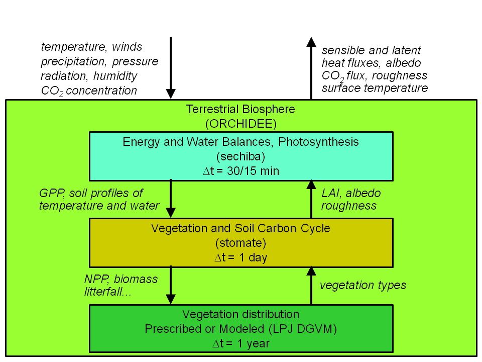
Figure 5 ORCHIDEE has no prescribed time resolution, nevertheless, the way processes were formalized largely reduces this flexibility. Four different time steps can be defined within the model. One time step, typically 30 minutes, defines the fast processes such as photosynthesis, autotrophic respiration, water and energy fluxes. A second time step controls the water routing in lakes and rivers. This is typically the same as the fast time step but can deviate slightly from it. A third time step, typically one day, controls the medium-fast processes such as heterotrophic respiration, carbon allocation within the plant and leaf area index. The final time step controls the slow processes which need only to be calculated once per year, such as vegetation dynamics, and ecosystem management.